Paper
Are you rushing
or dragging?
A Benchmark for Temporal Controllability in Text-to-Music Generation
Abstract—Text-to-music systems now produce high-fidelity audio from natural-language prompts, but applications that synchronize music to visual media require precise control over when musical events occur, not only what they sound like. We present TimingBench, a benchmark that measures temporal controllability: whether a generated clip delivers an instructed musical event such as an instrument entry, or a pause, and more, within a fixed tolerance of an instructed timestamp. TimingBench contributes three things: (i) a set of 250 prompts spanning single-event, multi-event, and tempo instructions, each carrying a machine-readable event schema; (ii) a deterministic, self-calibrated signal-processing evaluation pipeline that routes every instructed event to a purpose-built detector behind a cascade of rejection-only gates, so densely eventful music cannot score by luck; and (iii) a measurement of the pipeline's own localization error against human annotations (per-family median 8–218 ms), together with a human-annotated validation set, under construction, for independent detector evaluation. TimingBench turns a temporal instruction such as “bring in drums at exactly the sixth second” into a reproducible, apparatus-aware measurement. All scoring is reproducible; the benchmark is available at aalap-mvp.github.io/taan-timing-benchmark.
I. Introduction
Generative music models have advanced rapidly: systems such as MusicLM [1], MusicGen [2], Stable Audio [3], and commercial platforms (Suno, Udio, ElevenLabs Music, Google Lyria) render polished, prompt-conditioned audio in seconds. Evaluation practice, however, has concentrated on fidelity and global prompt adherence: Fréchet Audio Distance [4], CLAP-based text–audio similarity [5], and human preference, none of which asks directly whether the music does the right thing at the right time.
Temporal precision is not a niche concern. Music for film, advertising, games, and short-form video must align hits, entrances, and drops to picture, commonly within a few hundred milliseconds. A system that can produce “tense strings, and a drum entrance at exactly the sixth second” only if the entrance may drift by two seconds is not usable for synchronization work, no matter how good it sounds. Research systems have begun to address time-varying conditioning — melody or rhythm conditioning in MusicGen [2], time-varying controls in Music ControlNet [7], and symbolic/temporal conditioning in JASCO [8] but there has been no standardized way to measure whether any system, research or commercial, actually honors an explicit temporal instruction given in text.
Measuring this is harder than it appears. The evaluator must locate a specific musical event in generated audio whose style, mix, and instrumentation are unconstrained; it must not reward coincidental activity (dense arrangements contain onsets near every timestamp); it must distinguish “the model did it late” from “the model never did it”; and it must know its own measurement error, since a benchmark that cannot localize events more precisely than the tolerance it scores against is meaningless. Human annotation of every generated clip does not scale and is itself noisy for events without a crisp physical onset.
TimingBench addresses these requirements with three design commitments:
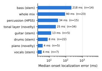
(1) Deterministic, self-calibrated measurement. Every scored number is produced by a deterministic signal-processing pipeline (source separation, onset statistics, spectral novelty, level analysis) with all thresholds in versioned configuration. The pipeline's own error is measured against human annotations and published per event family (Fig. 2); model-to-model differences smaller than the relevant measurement floor are treated as noise.
(2) False-positive–averse scoring. Every detection must pass a cascade of rejection gates (absence-before for entrances, persistence, local level change, semantic family evidence); an event that fails any gate scores as “not delivered.” This bounds what densely eventful music could earn by luck.
(3) Claim honesty. The benchmark separates timing claims from timbre claims. For instruments isolable by source separation, a credited event asserts that the named instrument moved on time; for arbitrary tonal layers, it asserts that a new tonal layer moved on time, with instrument identity verified at coarse family granularity by a separate mechanism and reported as its own metric.
This paper presents the benchmark and its measurement apparatus in full: the prompt and event schema (Sec. III), the deterministic evaluation pipeline and its family-specific detectors (Sec. IV), the calibration and validation that bound the pipeline's own measurement error (Sec. V), and a human-annotated validation set, under construction, for independent detector evaluation. Applying the benchmark to specific generation systems, and the resulting picture of temporal controllability in deployed text-to-music, is reported separately.
III. The Benchmark
A. Prompts and instruction schema
TimingBench contains 250 prompts in three families
(Table I): single-event prompts (100) request one timed event
(“Create a tense cinematic electronic track for exactly 30 seconds. Bring in drums at
exactly the 6th second.”); event-sequence prompts (100) request two to three ordered events
(silence until t1, entrance at t2, pause at t3, …); tempo prompts (50) request an exact BPM. Every
prompt requests exactly 30 s of instrumental audio. Prompts were authored from
templates spanning ~40 style descriptors (cinematic, orchestral, electronic, pop, jazz,
ambient, …) and nine instrument families, then manually reviewed. Each prompt carries a
machine-readable annotation: for every instructed event, the target text, an event kind
drawn from a closed vocabulary (instrument_entry, instrument_exit, music_start_after_silence, music_end, music_pause, mix_energy_increase), the
instructed time, and the tolerance. In total the set defines 399 timed events (287 entries,
59 exits, 27 silence-starts, 19 whole-mix ends/pauses, 7 energy increases) and 50 tempo
targets.
| Prompts (single / sequence / tempo) | 250 (100/100/50) |
| Timed events defined | 399 |
| Tempo targets | 50 |
| Event kinds | 6 |
| Style descriptors / instrument families | ~40 / 9 |
| Requested duration per clip | 30 s |
B. Corpus
To evaluate a system, each of the 250 prompts is submitted to it and the returned audio scored; a system may be sampled multiple times per prompt. Systems frequently ignore the duration instruction and return clips longer than the requested 30 s. All instructed times lie within the first 30 s, and the evaluator computes its per-clip reference statistics on the leading 35 s so that trailing material cannot shift calibrated thresholds; duration is itself an instruction and is reported as its own metric. Provider-side generation failures are excluded and disclosed per evaluated system.
IV. Evaluation Methodology
A. Overview
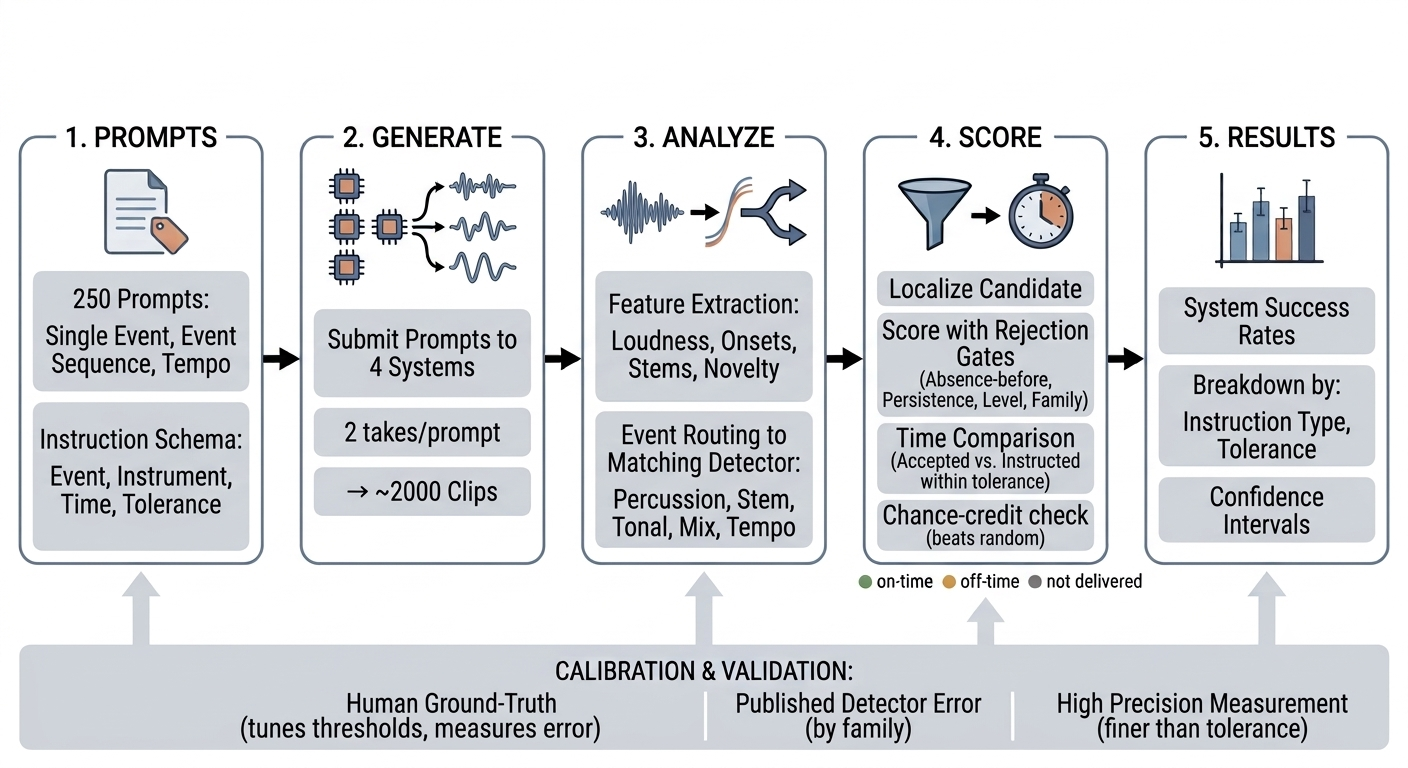
Fig. 1 summarizes scoring. Audio is decoded to 44.1 kHz mono, and a feature bank is computed on a common ~11.6 ms frame grid: mix RMS; full-band, harmonic, and percussive onset strength; harmonic–percussive separation; frequency-band envelopes; hybrid transformer source-separated stems (drums, bass, vocals, other, plus piano and guitar when required) [9], [10]; and a checkerboard-kernel spectral novelty curve over timbre and harmony features [13]. All decision thresholds are relative to the clip's or source's own measured loudness statistics; we verified that scoring is invariant (identical verdicts, onset shifts ≤ one frame) under −12 and −20 dB gain, so mastering level does not affect results.
Each instructed event is scored inside a search window of ±5 s around its instructed time, clamped to half the gap to the nearest sibling event so that one acoustic transition cannot satisfy two instructions. Failure of any gate yields the outcome none: “the model did not deliver the event” is a first-class result and counts against success, distinct from delivering it off-time.
B. Event-family detectors
Percussion. Drum and percussion events are scored on a rectified onset density: the trailing 1 s mean of the routed onset curve above its leading-window noise floor. This density rises at the first hit of a train and falls at the last, matching how human annotators mark such events; detections snap to the underlying accent for precision. The entrance-absence requirement is checked on the unrectified stem envelope so that quiet pre-existing percussion cannot be erased by rectification.
Stem-isolable instruments (bass, guitar, piano, vocals). Events are localized as sustained presence flips of the instrument's separated stem relative to its own loudness reference. Entrances require measured absence before the event at two scales (a whole-clip bound and a strict 3 s immediate window); exits require sustained absence after.
Tonal layers without a dedicated stem (strings, brass, synths, harp, …). Localization uses the spectral novelty curve (when); a harmonic-energy or register-band rise confirms the change is tonal (whether); and a semantic family gate supplies the who: the event's coarse instrument family (strings / brass / woodwinds / keys / plucked / vocals), embedded via a contrastive audio–text model [5] run in windows across the clip, must rise across the candidate and must have been quiet before it — the absence evidence that identity-blind novelty lacks. The audio–text model is used strictly as a rejection gate with fixed thresholds; it can veto a candidate but can never move one or create one. Families on which the embedding is unreliable for generated audio (synthesizers, pads) are exempted from the gate and disclosed as a limitation.
Whole-mix events. “Silence” is defined 35 dB below the clip's loud level with hysteresis. An ending is scored as two edges: a first edge — the last accent (snapped on the onset curves), an abrupt cut, or, for gradual fades with no stop instant, the point where audio falls 23 dB below the loud level — and a decay requirement: the mix must be musically gone within 3 s of the first edge and stay down. Pauses (identified from prompt wording) require the same edges but only a bounded 3 s quiet interval, after which music may resume; without this distinction every genuine pause would be rejected as a non-terminal breakdown.
Tempo. Clip tempo is estimated from the beat times produced by an RNN beat tracker with dynamic-Bayesian-network decoding [11]: inter-beat intervals are trimmed to their 5–95th percentile range (dropping pickup-bar artifacts at clip boundaries) and the clip tempo is the mean of their reciprocals. On synthetic references whose tempo is exact by construction (click tracks and drum patterns at 50–174 BPM, including off-grid targets), this estimator's error is at most 0.06% of target — two orders of magnitude below the strictest tolerance we report — so tempo is scored on pure percentage tolerances with no absolute floor. A tempo instruction is credited when the estimate falls within ±3% of the target; we additionally report a {2,3,5}% tolerance ladder, octave-equivalent accuracy over factors {⅓,½,1,2,3} following MIREX convention [14], and beat-to-beat stability statistics. Half/double-time renderings therefore count as failures under the headline criterion and are visible separately in the octave-equivalent rate.
C. Calibration and validation
Thresholds fall into three provenance classes, all documented in the released configuration: conventions (search window, tolerance ladder, the 3 s decay budget), calibrated constants fit on a purpose-built annotated development set with order-of-magnitude margins between accept and reject populations (presence floors, absence bounds, level-ratio gates), and a small number of few-shot constants calibrated on fewer examples (novelty confirmation, end-snap guards), which we subject to extra scrutiny: a sensitivity sweep re-scores the full annotated validation set with every fitted constant perturbed by ±10/±20% and disabled entirely. No new false credits appear anywhere within ±10%; all false credits at ±20% occur only when a constant is moved in its loosening direction, indicating margin-set rather than razor-tuned thresholds. Disabling each gate identifies which are load-bearing (each prevents specific false credits) versus redundant
Ground truth for validation comprises 148 events annotated by the authors by ear (entrances, exits, ends, pauses, silences, and negatives i.e. “the requested event never happens”) across all four systems' audio, plus a 52-event development set. Development audio is quarantined: every clip whose annotation influenced any code or threshold was regenerated fresh for the reported run, so the evaluation corpus is untouched by calibration. Running the exact scoring path over the 128 benchmark-conditions validation events yields the confusion profile in Table II and the per-detector localization floors in Fig. 2: the pipeline's residual score-inflating outcomes (6 false positives + 4 false credits of 128) are confined to documented failure classes, and every per-family measurement floor is far below the smallest model-to-model differences we report.
| Correct credits (on-time events credited) | 12 |
| Correct rejections (negatives rejected) | 49 |
| Correct non-credits (off-time/missing events) | 55 |
| Missed on-time events | 2 |
| False credits | 4 |
| False positives (event invented) | 6 |
D. A human-annotated validation set (in progress)
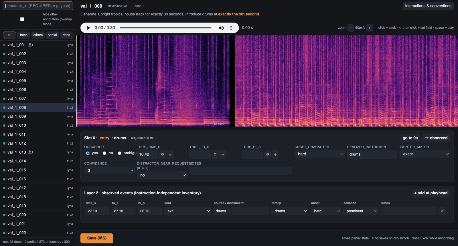
The author-labelled events above are sufficient to bound the pipeline's error, but a larger, independently-labelled set lets us characterize the detector at scale and on ears other than the designers'. We are therefore building a dedicated human-annotated validation set of 300 clips: 200 single-event (type 1) and 100 event-sequence (type 2) prompts, with audio generated by the two strongest in-distribution commercial systems, ElevenLabs v2 and Google Lyria. Each clip is labelled in a purpose-built interface (Fig. 3) that pairs an audio player with a zoomable log-mel spectrogram; the annotator clicks the spectrogram to set an onset time.
Labelling proceeds in two independent layers. Layer 1 (prompt adherence) records, for each instructed event, whether it occurred, its onset time, its onset character (hard, soft, or gradual), its salience, and its displacement from the prompt. Layer 2 (observed events) is an instruction-independent inventory: every audible event in the clip with its source/instrument, coarse family, onset, and salience, whether or not the prompt asked for it. Layer 1 measures what the model was told to do; Layer 2 captures the full event content, which is what lets us later separate genuine detections from coincidental activity. Guidelines are brief and fixed: onsets are marked at the first audible attack, using the same first-onset and gradual-fade conventions the detector is scored against, and every audible onset is marked regardless of the prompt.
This set is still being labelled. We therefore defer its dataset statistics (onset counts, distribution of onset types, rate of unprompted “extra” events) and, crucially, a detector-accuracy evaluation of our pipeline against these independent human labels to the complete-dataset release; both are in active scope and will be added once labelling finishes.
E. Chance-credit control
Busy music contains onsets near every timestamp. For every timed event we therefore re-score the same clip at 16 random instructed times (seeded, reproducible) with identical detectors and gates. The fraction credited, pchance, accompanies every event score: values near zero mean an on-time credit is real evidence of control rather than a coincidence of dense onsets. Reporting pchance with every credit, and re-scoring on low-pchance subsets, lets any comparison drawn with the benchmark discount events that busy arrangements could earn by luck.
F. Timing/timbre separation
For stem-isolable targets, a credit asserts the named instrument moved on time. For tonal-layer targets, the timing claim is family-level by construction; instrument identity is assessed separately (coarse-family audio–text evidence and reported as a timbre-match rate, never mixed into the timing score. This avoids both silently over-claiming identity and double-penalizing timing for timbre confusions, systems frequently render a requested exotic instrument as a near neighbor (e.g., a marimba request produces a piano-like timbre), which we treat as a timbre observation, not a timing failure.
V. Detector Evaluation
A. Measurement confidence
Every reported rate should be read against the instrument that produced it. Fig. 2 gives the per-family localization floors (median 8 ms for drum events through 218 ms for bass, reflecting attack sharpness and separation quality), and the tempo estimator's own error is at most 0.06% of target on exact-tempo synthetic references (Sec. IV); the validation confusion profile (Table II) bounds residual false credits at ~8% of labelled events, concentrated in documented classes (identity-ambiguous tonal layers, low-frequency bleed into the bass stem, sparse ambiguous onsets). Because rejection gates dominate the design, the benchmark's known bias is conservative: true recall is slightly understated, uniformly across whatever system is measured. The per-family floors and the ~8% residual false-credit rate together bound what the apparatus can and cannot resolve, and any comparison drawn with the benchmark must be read against them; a forthcoming release adds an independent human-annotated validation set (Sec. IV-D) for a larger-scale detector evaluation.
VI. Limitations and Future Work
Scope of identity claims. For stemless tonal layers, timing credits are family-level; fine-grained instrument identity on generated audio remains an open verification problem. The current audio–text embeddings are unreliable for synthesizers and audio with heavy effects (fx) and blur related acoustic families, and audio-language models, while promising as semantic verifiers, show weak temporal grounding [15]. We restrict all learned components to rejection-only roles and publish their exemptions.
Annotation variance. Some musical events have no single correct instant (gradual fades, spread attacks, sparse note trains); our conventions (first audible onset; fade endings scored where audio is musically gone) are documented choices, and inter-annotator variance on such events bounds achievable agreement for any evaluator.
Prompt coverage. The prompt set emphasizes clearly measurable events by design; instructions whose realization is intrinsically ambiguous (dense sub-second event spacing, vague removals) are underrepresented, a deliberate trade of coverage for measurement validity.
Extensions. Natural next steps include: evaluating research systems with explicit temporal conditioning; extending the schema to synchronization-style briefs (multiple aligned cues per clip); integrating audio-language models as calibrated semantic verifiers once their temporal grounding matures; and closing the loop with generation systems that plan events symbolically before synthesis, for which this benchmark provides a direct target.
VII. Conclusion
TimingBench turns “bring in drums at exactly the sixth second” into a measurement: a deterministic, self-calibrated evaluation of temporal instruction following, with published per-family measurement floors, a chance-credit control, and a human-annotated validation set for detector evaluation. It makes millisecond-accurate temporal controllability — the capability that music-for-media applications require — measurable and reproducible; applying it across generation systems is the subject of companion work.
References
- A. Agostinelli et al., “MusicLM: Generating music from text,” arXiv:2301.11325, 2023.
- J. Copet et al., “Simple and controllable music generation,” in NeurIPS, 2023.
- Z. Evans et al., “Fast timing-conditioned latent audio diffusion,” in ICML, 2024.
- K. Kilgour, M. Zuluaga, D. Roblek, and M. Sharifi, “Fréchet audio distance: A metric for evaluating music enhancement algorithms,” in INTERSPEECH, 2019.
- Y. Wu, K. Chen, T. Zhang, Y. Hui, T. Berg-Kirkpatrick, and S. Dubnov, “Large-scale contrastive language-audio pretraining with feature fusion and keyword-to-caption augmentation,” in ICASSP, 2023.
- R. Huang et al., “Make-An-Audio: Text-to-audio generation with prompt-enhanced diffusion models,” in ICML, 2023.
- S.-L. Wu, C. Donahue, S. Watanabe, and N. J. Bryan, “Music ControlNet: Multiple time-varying controls for music generation,” IEEE/ACM TASLP, 2024.
- O. Tal, A. Ziv, I. Gat, F. Kreuk, and Y. Adi, “Joint audio and symbolic conditioning for temporally controlled text-to-music generation,” in ISMIR, 2024.
- A. Défossez, “Hybrid spectrogram and waveform source separation,” in ISMIR MDX Workshop, 2021.
- S. Rouard, F. Massa, and A. Défossez, “Hybrid transformers for music source separation,” in ICASSP, 2023.
- S. Böck, F. Korzeniowski, J. Schlüter, F. Krebs, and G. Widmer, “madmom: A new Python audio and music signal processing library,” in ACM Multimedia, 2016.
- B. McFee et al., “librosa: Audio and music signal analysis in Python,” in SciPy, 2015.
- J. Foote, “Automatic audio segmentation using a measure of audio novelty,” in IEEE ICME, 2000.
- C. Raffel et al., “mir_eval: A transparent implementation of common MIR metrics,” in ISMIR, 2014.
- S. Sakshi et al., “MMAU: A massive multi-task audio understanding and reasoning benchmark,” in ICLR, 2025.
- Q. Yang et al., “AIR-Bench: Benchmarking large audio-language models via generative comprehension,” in ACL, 2024.